Model selection

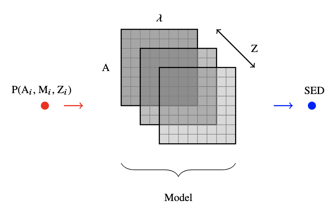
Since the stellar particles within hydrodynamical simulations represent simple stellar populations (SSPs), we can leverage stellar population synthesis (SPS) to infer the spectral energy distributions (SEDs) of the stellar particles within the simulation. This SED will then describe the brightness of a given particle as a function of wavelength. There are many uncertainties associated with SPS, and different works make different assumptions about the physics that they are modelling. While the exact form of the SEDs will vary depending on the physical assumptions, all of them model the evolution of SEDs as two-dimensional arrays containing ages on one axis and wavelengths/frequencies on the other. These SEDs are also metallicity-dependent, so we need one array file for each metallicity. For a given stellar particle, PyMGal reads its physical properties such as age, mass, and metallicity. It then interpolates the model files, maps the particle to an SED that most closely matches its physical properties, and then scales the SED based mass. An illustration of this process can be found below for a stellar particle P, where we denote age by A, metallicity by Z, mass by M, and wavelengths by λ.

For best results, you should ensure that the metallicity range in your models encompasses the entire metallicity range of stellar particles. If this is not the case, particles with metallicity that falls beyond the model range will be mapped to the closest boundary, which may introduce bias.

The SSP_models object

You may change the stellar population model to best fit your research goals. Note that while the default model comes with its full metallicity range, this may not be true of every model. If the model files you want are not already provided, you may need to create your own. If you need to study the contents of the .model files in order to replicate them, it might be helpful to convert them to .fits first and then look at them that way. Model files can also be read in .txt, .fits, or .ised format (.ised being the original format in which the BC03 models were distributed).

from pymgal import SSP_models, MockObservation

model_type = "bc03"
model = SSP_models(model_type, IMF="chab")
obs = MockObservation("/path/to/snapshot", [x_c, y_c, z_c, r], params = {"model": model})

SSP_models parameters

The code below shows the full list of options for the SSP_models class, as well as how you can print its docstring for more details.

model = SSP_models(model_file, IMF="chab", metal=[list], is_ised=False, is_fits=False,
is_ascii=False, has_masses=False, units='a', age_units='gyrs', nsample=None, quiet=True, model_dir=None)

print(SSP_models.__doc__)

The most important are the model_file and the initial mass function (IMF). If you want to only look at some metallicities, specify them with the metal parameter. If you want to specify your own model in a .txt file, .fits file, or .ised file, make sure to set is_ascii=True, is_fits=True, or is_ised=True, respectively. You may also want to specify your own custom model directory by setting model_dir=”/path/to/your/models”

Available models

PyMGal borrows the .model format from EzGal, which allows it to support various types of models from different works. Below is a list of models that were created for the EzGal package. They are BC03 from Bruzual & Chalot (2003), M05 from Maraston (2005), CB07 from Charlot & Bruzual (2007), BaSTI from Percival et al. (2009), C09 for the FSPS models from Conroy et al. (2009) and P2 for the PEGASE2 set from Fioc & Rocca-Volmerange (1997).

For more details on these, consult the EzGal paper and/or website (http://www.baryons.org/ezgal). If you’d like to download more models, you can access them here: http://www.baryons.org/ezgal/download.php. Make sure to cite the EzGal authors and model authors. We include a table of all the EzGal libraries that are compatible with PyMGal, as well as their properties such as the number of ages, the number of metallicities, and the range of these metallicities.

Category	Available IMFs	Metallicity range (Z/Z_solar)	No. metallicities	No. ages
BC03	Chabrier, Salpeter	0.005 - 2.5	6	221
M05	Kroupa, Salpeter	0.05-3.5	5	68
CB07	Chabrier, Salpeter	0.005 - 2.5	6	221
C09	Chabrier, Kroupa, Salpeter	0.01 - 1.5	22	189
P09	Kroupa	0.005 - 2.5	10	56
P2	Salpeter	0.005 - 5	7	69

Dust functions

If you want to model the effect of dust in the SEDs, PyMGal features two dust functions that are described in Charlot and Fall (2000) or Calzetti et al. (2000). This will dim the SEDs based on the physical law you select. You can call these functions by creating a dust object and passing it to a MockObservation.

You can also incorporate the effect of dust extinction along the line of sight. PyMGal estimates this effect by calculating the column density of gas particles within a pixel N_g (i.e. gas mass divided by pixel area). It then multiplies this column density by the opacity kappa, which the user can choose to match their research needs. The brightnesses are then dimmed by a factor of e^(-kappa*N_g).

from pymgal import MockObservation, SSP_models, dusts

calzetti_dust = dusts.calzetti()
obs_calzetti = MockObservation("/path/to/snapshot", [x_c, y_c, z_c, r], params = {"dustf": calzetti_dust})

charlot_fall_dust = dusts.charlot_fall()
obs_charlot_fall = MockObservation("/path/to/snapshot", [x_c, y_c, z_c, r], params = {"dustf": charlot_fall_dust})

los_dust = dusts.los_extinction(kappa=10)
obs_los_dust = MockObservation("/path/to/snapshot", [x_c, y_c, z_c, r], params = {"dustf_los":dust_los})

You may use whichever combination of dust best suits your research needs. This may include both “dustf” and “dustf_los”, neither, or only one of the two. Typically using both will produce the most realistic observations (assuming kappa is given an appropriate value), but line of sight dust exctinction will be more computationally expensive.

In the above line of sight dust treatment, we set kappa=10. This means that the opacity will be treated as a constant value of 10 cm^2/g. However, you can also change this value or infer it from the gas properties by setting kappa=”kappa_e” (deriving the opacity from electron scattering), “kappa_k” (Kramer’s opacity for free-free/bound-free absorption), “kappa_m” (molecular opacity), “kappa_h” (negative hydrogen ion opacity), “kappa_rad” (the total radiative opacity considering the effects from the previous 4 sources), or “kappa_d” (dust opacity - still a work in progress).